44 data labels on excel chart

how to add data labels into Excel graphs - storytelling with data There are a few different techniques we could use to create labels that look like this. Option 1: The "brute force" technique. The data labels for the two lines are not, technically, "data labels" at all. A text box was added to this graph, and then the numbers and category labels were simply typed in manually. › documents › excelHow to add data labels from different column in an Excel chart? This method will guide you to manually add a data label from a cell of different column at a time in an Excel chart. 1. Right click the data series in the chart, and select Add Data Labels > Add Data Labels from the context menu to add data labels. 2. Click any data label to select all data labels, and then click the specified data label to select it only in the chart.

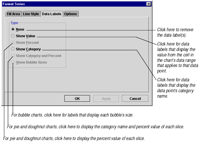
Change the format of data labels in a chart You can add a built-in chart field, such as the series or category name, to the data label. But much more powerful is adding a cell reference with explanatory text or a calculated value. Click the data label, right click it, and then click Insert Data Label Field. If you have selected the entire data series, you won't see this command.

Data labels on excel chart

blog.hubspot.com › marketing › how-to-build-excel-graphHow to Make a Chart or Graph in Excel [With Video Tutorial] Sep 08, 2022 · Enter your data into Excel. Choose one of nine graph and chart options to make. Highlight your data and click 'Insert' your desired graph. Switch the data on each axis, if necessary. Adjust your data's layout and colors. Change the size of your chart's legend and axis labels. Change the Y-axis measurement options, if desired. Create Dynamic Chart Data Labels with Slicers - Excel Campus Step 6: Setup the Pivot Table and Slicer. The final step is to make the data labels interactive. We do this with a pivot table and slicer. The source data for the pivot table is the Table on the left side in the image below. This table contains the three options for the different data labels. Excel tutorial: How to use data labels Data labels are used to display source data in a chart directly. They normally come from the source data, but they can include other values as well, as we'll see in in a moment. Generally, the easiest way to show data labels to use the chart elements menu. When you check the box, you'll see data labels appear in the chart.

Data labels on excel chart. How to I rotate data labels on a column chart so that they are ... To change the text direction, first of all, please double click on the data label and make sure the data are selected (with a box surrounded like following image). Then on your right panel, the Format Data Labels panel should be opened. Go to Text Options > Text Box > Text direction > Rotate Excel Charts - Aesthetic Data Labels - tutorialspoint.com To place the data labels in the chart, follow the steps given below. Step 1 − Click the chart and then click chart elements. Step 2 − Select Data Labels. Click to see the options available for placing the data labels. Step 3 − Click Center to place the data labels at the center of the bubbles. Format a Single Data Label How to Use Cell Values for Excel Chart Labels - How-To Geek Select the chart, choose the "Chart Elements" option, click the "Data Labels" arrow, and then "More Options." Uncheck the "Value" box and check the "Value From Cells" box. Select cells C2:C6 to use for the data label range and then click the "OK" button. The values from these cells are now used for the chart data labels. peltiertech.com › prevent-overlapping-data-labelsPrevent Overlapping Data Labels in Excel Charts - Peltier Tech May 24, 2021 · Here is the chart after running the routine, without allowing any overlap between labels (OverlapTolerance = zero).All labels can be read, but the space between them is greater than needed (you could almost stick another label between any two adjacent labels here), and some labels have moved far from the points they label.

Data Labels in Excel Pivot Chart (Detailed Analysis) The data label is a marker on the Excel Chart, where this marker is linked with the data in the Table and updates when the data is updated. A data label is such a useful feature using which can give you the info about the data or data series instantly. Which part of the chart denotes which data can be easily distinguished through the Data Labels. Excel Chart Data Labels - Microsoft Community Right-click a data point on your chart, from the context menu choose Format Data Labels ..., choose Label Options > Label Contains Value from Cells > Select Range. In the Data Label Range dialog box, verify that the range includes all 26 cells. When I paste your data into a worksheet, the XY Scatter data is in A2:B27, and the data labels are in ... Edit titles or data labels in a chart - support.microsoft.com On a chart, click one time or two times on the data label that you want to link to a corresponding worksheet cell. The first click selects the data labels for the whole data series, and the second click selects the individual data label. Right-click the data label, and then click Format Data Label or Format Data Labels. › excel-chart-verticalExcel Chart Vertical Axis Text Labels • My Online Training Hub So all we need to do is get that bar chart into our line chart, align the labels to the line chart and then hide the bars. We’ll do this with a dummy series: Copy cells G4:H10 (note row 5 is intentionally blank) > CTRL+C to copy the cells > select the chart > CTRL+V to paste the dummy data into the chart.

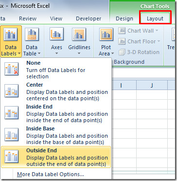
Add a DATA LABEL to ONE POINT on a chart in Excel Click on the chart line to add the data point to. All the data points will be highlighted. Click again on the single point that you want to add a data label to. Right-click and select ' Add data label ' This is the key step! Right-click again on the data point itself (not the label) and select ' Format data label '. How to Add Data Labels to Scatter Plot in Excel (2 Easy Ways) - ExcelDemy 2 Methods to Add Data Labels to Scatter Plot in Excel 1. Using Chart Elements Options to Add Data Labels to Scatter Chart in Excel 2. Applying VBA Code to Add Data Labels to Scatter Plot in Excel How to Remove Data Labels 1. Using Add Chart Element 2. Pressing the Delete Key 3. Utilizing the Delete Option Conclusion Related Articles How to Add Two Data Labels in Excel Chart (with Easy Steps) Select the data labels. Then right-click your mouse to bring the menu. Format Data Labels side-bar will appear. You will see many options available there. Check Category Name. Your chart will look like this. Now you can see the category and value in data labels. Read More: How to Format Data Labels in Excel (with Easy Steps) Things to Remember How to Add Data Labels in Excel - Excelchat | Excelchat After inserting a chart in Excel 2010 and earlier versions we need to do the followings to add data labels to the chart; Click inside the chart area to display the Chart Tools. Figure 2. Chart Tools Click on Layout tab of the Chart Tools. In Labels group, click on Data Labels and select the position to add labels to the chart. Figure 3.

Adding rich data labels to charts in Excel 2013 | Microsoft ...

Excel charts: add title, customize chart axis, legend and data labels Click anywhere within your Excel chart, then click the Chart Elements button and check the Axis Titles box. If you want to display the title only for one axis, either horizontal or vertical, click the arrow next to Axis Titles and clear one of the boxes: Click the axis title box on the chart, and type the text.

How to add or move data labels in Excel chart?

How to insert or add axis labels in Excel 350 charts (with Example)? Adding axis title labels to Excel chart In Microsoft Excel, select your data and hit Insert, then from the Ribbon pick the scatter chart. A simple chart will be rendered. Now, go ahead and click on your chart figure external border. You'll notice three buttons popping up at the upper right side of ...

Change the format of data labels in a chart

Custom Chart Data Labels In Excel With Formulas - How To Excel At Excel Follow the steps below to create the custom data labels. Select the chart label you want to change. In the formula-bar hit = (equals), select the cell reference containing your chart label's data. In this case, the first label is in cell E2. Finally, repeat for all your chart laebls.

How to set and format data labels for Excel charts in C#

› how-to-create-excel-pie-chartsHow to Make a Pie Chart in Excel & Add Rich Data Labels to ... Sep 08, 2022 · In this article, we are going to see a detailed description of how to make a pie chart in excel. One can easily create a pie chart and add rich data labels, to one’s pie chart in Excel. So, let’s see how to effectively use a pie chart and add rich data labels to your chart, in order to present data, using a simple tennis related example.

Example: Charts with Data Labels — XlsxWriter Documentation

What are the Chart elements in Excel | Easy Learn Methods After creating a chart, you can add new chart elements in excel like chart titles, axis titles, legends, data labels, grid lines, etc. Many of them are optional and you always can remove or add them according to your needs, default displays the most essential elements when creating the chart. You can also change the formatting of existing ones.

Change Chart Data Labels : Chart Data « Chart « Microsoft ...

Add data labels and callouts to charts in Excel 365 - EasyTweaks.com Excel also gives you the option of formatting the data labels to suit your desired look if you don't like the default. To make changes to the data labels, right-click within the chart and select the "Format Labels" option. Some of the formatting options you will have include; changing the label position, changing its alignment angle, and many more.

Custom data labels in a chart

› excel-pie-chartExcel Pie Chart - How to Create & Customize? (Top 5 Types) #Adding Data Labels. We will customize the Pie Chart in Excel by Adding Data Labels. Scenario 1: The procedure to add data labels are as follows: Click on the Pie Chart > click the ‘+’ icon > check/tick the “Data Labels” checkbox in the “Chart Element” box > select the “Data Labels” right arrow > select the “Outside End” option.

Align data labels in a graph so they are all along the same ...

support.microsoft.com › en-us › officeAdd or remove data labels in a chart - support.microsoft.com Add data labels to a chart Click the data series or chart. To label one data point, after clicking the series, click that data point. In the upper right corner, next to the chart, click Add Chart Element > Data Labels. To change the location, click the arrow, and choose an option. If you want to ...

microsoft excel - Prevent two sets of labels from overlapping ...

How To Add Data Labels In Excel - dark-team.info To get there, after adding your data labels, select the data label to format, and then click chart elements > data labels > more options. After picking the series, click the data point you want to label. Source: temotips.blogspot.com. Using excel chart element button to add axis labels. Click the chart to show the chart elements button.

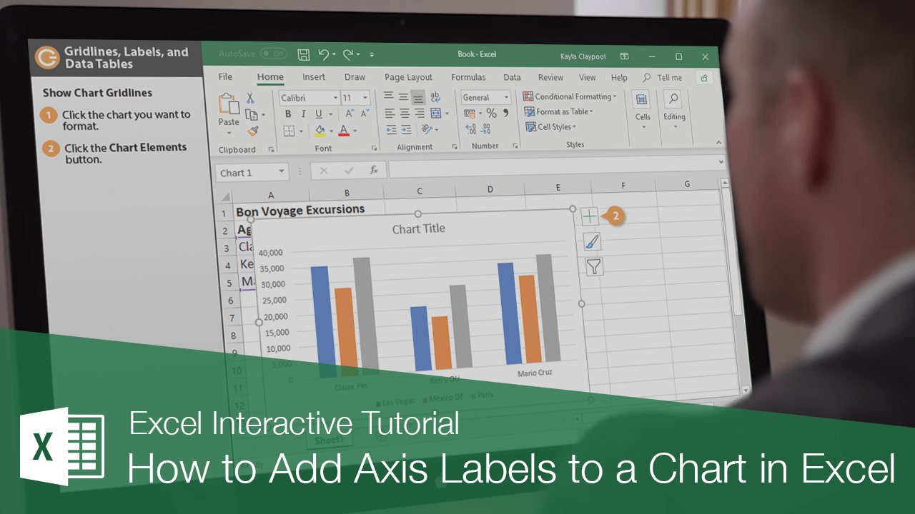
How to Add Axis Labels to a Chart in Excel | CustomGuide

How To Use Dynamic Data Labels To Create Interactive Excel Charts To create a column chart with dynamic data labels, you need to follow these given steps. Select the data & Create a Combo Chart. Now select the column chart for revenue data and a line chart with marker for data labels. Add Data Labels to the Line Chart With Marker. After then remove the Line Color and Marker Color.

Excel 2010: Show Data Labels In Chart

How to Add Data Labels to an Excel 2010 Chart - dummies On the Chart Tools Layout tab, click Data Labels→More Data Label Options. The Format Data Labels dialog box appears. You can use the options on the Label Options, Number, Fill, Border Color, Border Styles, Shadow, Glow and Soft Edges, 3-D Format, and Alignment tabs to customize the appearance and position of the data labels.

Is there a way to add data labels as percentages on the ...

Move data labels - support.microsoft.com Right-click the selection > Chart Elements > Data Labels arrow, and select the placement option you want. Different options are available for different chart types. For example, you can place data labels outside of the data points in a pie chart but not in a column chart.

Placing Chart Data Labels – Daily Dose of Excel

Chart.ApplyDataLabels method (Excel) | Microsoft Learn Applies data labels to all the series in a chart. Syntax expression. ApplyDataLabels ( Type, LegendKey, AutoText, HasLeaderLines, ShowSeriesName, ShowCategoryName, ShowValue, ShowPercentage, ShowBubbleSize, Separator) expression A variable that represents a Chart object. Parameters Example

Custom data labels in a chart

Labels in a Scatter Chart - Microsoft Community I have a scatter chart with data points in the chart. The data points have lables. In addtion to these labels, I would like to place my cursor on a particular data point and it would show the contents of a particular cell. This would be addtional information about the data point but only shown when I place my cursor over it. This is is in ...

Change color of data label placed, using the 'best fit ...

How to add or move data labels in Excel chart? - ExtendOffice To add or move data labels in a chart, you can do as below steps: In Excel 2013 or 2016. 1. Click the chart to show the Chart Elements button . 2. Then click the Chart Elements, and check Data Labels, then you can click the arrow to choose an option about the data labels in the sub menu. See screenshot: In Excel 2010 or 2007. 1. click on the chart to show the Layout tab in the Chart Tools group. See screenshot: 2.

Format Data Labels in Excel- Instructions - TeachUcomp, Inc.

Excel tutorial: How to use data labels Data labels are used to display source data in a chart directly. They normally come from the source data, but they can include other values as well, as we'll see in in a moment. Generally, the easiest way to show data labels to use the chart elements menu. When you check the box, you'll see data labels appear in the chart.

Data labels on Excel charts « projectwoman.com

Create Dynamic Chart Data Labels with Slicers - Excel Campus Step 6: Setup the Pivot Table and Slicer. The final step is to make the data labels interactive. We do this with a pivot table and slicer. The source data for the pivot table is the Table on the left side in the image below. This table contains the three options for the different data labels.